bootstrapping method: an approach for a youngster literacy

In this article we will explore how to employ the bootstrapping method to estimate the parameters of an unobserved population function. We then apply this approach to analyze the exchange rates of EUR/USD- which is among the most liquid currency pairs in the foreign-exchange market. Our primary software tool is MATLAB R2022b, and we also reference Bradley Efron’s foundational work on bootstrap techniques.

1. resources-motivation

GROK.COM | as a practical guide to help structure and brainstorm each step of our data-analysis worflow.
Bradley Efron’s Original Papers on Bootstrap |to provide theoretical underpinning and justification for resampling.
MATLAB R2022b| as the computational environment to run the simulations.

Why BOOTSTRAPING? In many real scenearios (especially in financial markets) we cannot reliably assume a particular parametric form (e.g., Gaussian) for our data. Instead this method allow us to «resample» from the observed dataset itself to approximate confidence intervals, estimate bias, and measure the variability of any statistic.

So, as forecasting volatility is crucial for risk management, dynamic position sizing, and developing robust trading strategies. Traditional econometric approaches as GARCH assume specific parametric distributions, which often fail to capture heavy tails and skweness observed in financial data. That’s why here we apply the bootstrapping method for ditributional inference and then compare four ML (Machine Learning) models:

Bagging (Bootstrap Aggregation of decision trees).
Random Forest.
Suppor-Vector Regression (SVR) with an RBF kernel.
Feed-forward Neural Network (NN) with a single hidden layer.

Our dataset consists of daily closing prices of EUR/USD, which we turn into log-returns. Using MATLAB R2022b, we perfomr bootstrap analysis to characterize distributional properties (mean, variance, skewness, kurtosis) and then construct a forecasying task for 5-day realized volatility.

Aslo, note that each model is trained on 80% of data and test on the remaining 20% using RMSE, MAE and R2 as evaluation metrics. And finally, as an addition we extract predictor importance from Random Forest model to see which lagged returns matter most.

2. distributional analysis of EUR/USD log-returns

Before forecasting volatility, it’s essential to understand the distributional characteristics of daily returns. We first compute log-returns and then apply a bootstrap procedure.

set(groot, 'DefaultAxesFontName', 'Lucida Console');
set(groot, 'DefaultTextFontName', 'Lucida Console');
set(groot, 'DefaultAxesFontSize', 10);
set(groot, 'DefaultTextFontSize', 10);


clear; close all; clc; rng default        % Limpia variables, cierra figuras y fija la semilla

% =========================================================================
% 1. CARGA DE DATOS Y ESTADÍSTICAS BÁSICAS
% =========================================================================
% Carga el archivo de precios EUR/USD y calcula rendimientos logarítmicos
load eurusd.txt
x = diff(log(eurusd));        % Rendimientos logarítmicos
n = numel(x);                  % Número de observaciones
mu = mean(x);                  % Media muestral
sigma2 = var(x);               % Varianza muestral
sigma = std(x);                % Desviación típica muestral

% =========================================================================
% 2. VISUALIZACIÓN DE LA DISTRIBUCIÓN DE RENDIMIENTOS
% =========================================================================
% Grafica la CDF empírica junto con la CDF normal ajustada
figure;
[h, ~] = cdfplot(x);           % CDF empírica
hold on;
xv = linspace(min(x), max(x));
plot(xv, normcdf(xv, mu, sigma), 'r-', 'LineWidth', 2);
legend('Distribución Empírica', 'Distribución Normal', 'Location', 'best');
title('Comparación de la Distribución Empírica y Normal');
xlabel('Rendimientos Logarítmicos');
ylabel('Probabilidad Acumulada');
hold off;

% =========================================================================
% 3. PRUEBA DE NORMALIDAD (LILLIEFORS)
% =========================================================================
% Comprueba si los rendimientos provienen de una distribución normal
[h_norm, p_norm] = lillietest(x);
if h_norm == 0
    disp('No se rechaza la hipótesis de normalidad (p > 0.05)');
else
    disp('Se rechaza la hipótesis de normalidad (p < 0.05)');
end

% =========================================================================
% 4. INTERVALOS DE CONFIANZA TEÓRICOS (95%)
% =========================================================================
% Calcula intervalos de confianza usando la distribución normal y chi-cuadrado
ci_mu_teorico = [ mu + icdf('norm', 0.025, 0, 1) * sigma / sqrt(n), ...
                  mu + icdf('norm', 0.975, 0, 1) * sigma / sqrt(n) ];
ci_sigma2_teorico = [ (n - 1) * sigma2 / icdf('chi2', 0.975, n - 1), ...
                      (n - 1) * sigma2 / icdf('chi2', 0.025, n - 1) ];

fprintf('\nIC 95%% de la media (teórico): [%.6e, %.6e]\n', ci_mu_teorico(1), ci_mu_teorico(2));
fprintf('IC 95%% de la varianza (teórico): [%.6e, %.6e]\n', ci_sigma2_teorico(1), ci_sigma2_teorico(2));

% =========================================================================
% 5. BOOTSTRAP PARA MEDIA Y VARIANZA
% =========================================================================
% Genera B = 1000 réplicas bootstrap para estimar sesgo, error y IC
rng('default');               % Asegura reproducibilidad
num_bootstrap = 1000;
boot_mu     = bootstrp(num_bootstrap, @mean,    x);
boot_sigma2 = bootstrp(num_bootstrap, @var,     x);

% Calculo de intervalos de confianza percentil 2.5–97.5
ci_mu_boot     = prctile(boot_mu,     [2.5, 97.5]);
ci_sigma2_boot = prctile(boot_sigma2, [2.5, 97.5]);

% Cálculo de sesgo y error estándar de los estimadores bootstrap
bias_mu     = mean(boot_mu)     - mu;
se_mu       = std(boot_mu);
bias_sigma2 = mean(boot_sigma2) - sigma2;
se_sigma2   = std(boot_sigma2);

fprintf('\nIC 95%% de la media (bootstrap): [%.6e, %.6e]\n', ci_mu_boot(1), ci_mu_boot(2));
fprintf('Sesgo (media): %.6e, SE (media): %.6e\n', bias_mu, se_mu);
fprintf('\nIC 95%% de la varianza (bootstrap): [%.6e, %.6e]\n', ci_sigma2_boot(1), ci_sigma2_boot(2));
fprintf('Sesgo (varianza): %.6e, SE (varianza): %.6e\n', bias_sigma2, se_sigma2);

% =========================================================================
% 6. VISUALIZACIÓN DE LAS DISTRIBUCIONES BOOTSTRAP
% =========================================================================
figure;
subplot(2,1,1);
histogram(boot_mu, 30);
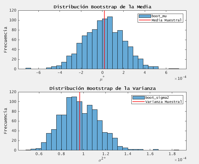
title('Distribución Bootstrap de la Media');
xlabel('\mu^*');
ylabel('Frecuencia');
xline(mu, 'r', 'LineWidth', 2, 'DisplayName', 'Media Muestral');
legend;

subplot(2,1,2);
histogram(boot_sigma2, 30);
title('Distribución Bootstrap de la Varianza');
xlabel('\sigma^2^*');
ylabel('Frecuencia');
xline(sigma2, 'r', 'LineWidth', 2, 'DisplayName', 'Varianza Muestral');
legend;

% =========================================================================
% 7. ANÁLISIS DE ASIMETRÍA Y CURTOSIS CON BOOTSTRAP
% =========================================================================
% Calcula asimetría y curtosis muestral, y sus IC bootstrap
skewness_sample = skewness(x);
kurtosis_sample = kurtosis(x);
boot_skewness   = bootstrp(num_bootstrap, @skewness, x);
boot_kurtosis   = bootstrp(num_bootstrap, @kurtosis, x);
ci_skewness     = prctile(boot_skewness, [2.5, 97.5]);
ci_kurtosis     = prctile(boot_kurtosis, [2.5, 97.5]);

fprintf('\nAsimetría muestral: %.6f (IC 95%%: [%.6f, %.6f])\n', skewness_sample, ci_skewness(1), ci_skewness(2));
fprintf('Curtosis muestral: %.6f (IC 95%%: [%.6f, %.6f])\n', kurtosis_sample, ci_kurtosis(1), ci_kurtosis(2));

figure;
subplot(2,1,1);
histogram(boot_skewness, 30);
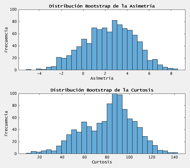
title('Distribución Bootstrap de la Asimetría');
xlabel('Asimetría');
ylabel('Frecuencia');

subplot(2,1,2);
histogram(boot_kurtosis, 30);
title('Distribución Bootstrap de la Curtosis');
xlabel('Curtosis');
ylabel('Frecuencia');

2.2. key-results

We have obtained the following results:

Se rechaza la hipótesis de normalidad (p < 0.05)

IC 95% de la media (teórico): [-3.567200e-04, 3.946739e-04]
IC 95% de la varianza (teórico): [9.161672e-05, 1.020795e-04]

IC 95% de la media (bootstrap): [-3.559769e-04, 3.707507e-04]
Sesgo (media): -6.451899e-06, SE (media): 1.900627e-04

IC 95% de la varianza (bootstrap): [6.684009e-05, 1.303464e-04]
Sesgo (varianza): 1.431490e-07, SE (varianza): 1.720387e-05

Asimetría muestral: 2.851049 (IC 95%: [-2.243697, 6.599361])
Curtosis muestral: 87.927355 (IC 95%: [34.965756, 120.904841])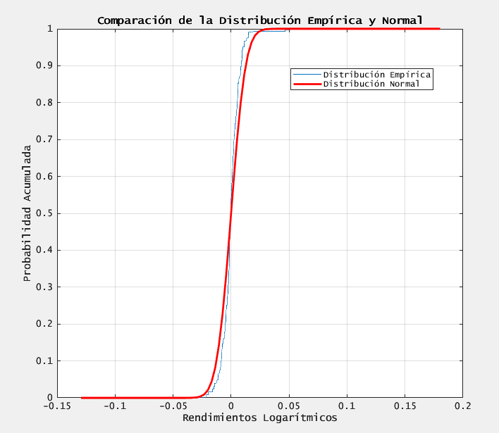

Among the results obtained we can settle the following statements:

we reject normality, confirming heavy tails and mild skew in the log-returns.
both methods agree that the mean is essentialy zero.
bootstrap CIs are slightly narrower.
significant excess kurtosis- far above 3- indicates frequent large shocks (both positive and negative).

3. volatility forecasting- task

Now that we understand its distributional properties, we move to forecasting 5-day realized volatility.

3.1. COMPUTE 5-DAY REALIZED VOLATILITY

% 3.1 Define the target: 5-day rolling variance
w = 5;                             
vol = movvar(x, w);   % realized volatility over 5-day window

3.2. CONSTRUCT LAGGED PREDICTORS

% 3.2 Build predictor matrix Xmat: lags 1 to 5
maxLag = 5;
Xmat = zeros(numel(vol) - maxLag, maxLag);
for L = 1:maxLag
    Xmat(:,L) = x(maxLag - L + 1 : end - L);
end
Y = vol(maxLag + 1 : end);  % corresponds to vol(6:end)

% 3.3 Name each column for later plotting
Xtrain = arrayfun(@(i) sprintf('Lag_%d', i), 1:maxLag, 'UniformOutput', false);

% 3.4 Standardize predictors (zero mean, unit variance)
Xmat_mu    = mean(Xmat);
Xmat_sigma = std(Xmat);
Xmat       = (Xmat - Xmat_mu) ./ Xmat_sigma;

Each row of Xmat is [rt-1, rt-2, rt-3, rt-4, rt-5].

Standarization ensures all lags are on the same scale which is essential to SVR and NN in particular.

3.3. TRAIN-split

% 3.5 Split data: 80% training, 20% test
cv = cvpartition(numel(Y), 'HoldOut', 0.2);
idxTr = training(cv);
idxTe = test(cv);
Xtr = Xmat(idxTr, :);   Ytr = Y(idxTr);
Xte = Xmat(idxTe, :);   Yte = Y(idxTe);

We hold out the last 20% of data for out-of sample evaluation.

The first 80% is used for model fitting and hyperparameter selection.

4. training machine-learning models

We now train four distinct models on (Xtr, Ytr) and generate forecast on Xte.

4.1. BAGGIN

% 4.1 Bagging: ensemble of regression trees via bootstrap
mdlBag = fitrensemble(Xtr, Ytr, 'Method', 'Bag');
YhatBag = predict(mdlBag, Xte);

b- Creates multiple decision trees trained on bootstrap samples, then averages their predictions.

4.2. RANDOM FOREST

% 4.2 Random Forest with out-of-bag predictor importance
numTrees = 200;
rf = TreeBagger(numTrees, Xtr, Ytr, 'Method', 'regression', ...
                'NumPredictorsToSample', ceil(maxLag/2), ...
                'OOBPredictorImportance', 'on');
[YhatRF, stdRF] = predict(rf, Xte);
YhatRF = double(YhatRF);  % convert cell array to numeric

rf- Uses 200 trees; each split considers a random subset of 3 predictors.

4.3. SUPPORT-VECTOR REGRESSION (SVR)

% 4.3 SVR with Gaussian (RBF) kernel, automatic scaling
mdlSVR = fitrsvm(Xtr, Ytr, 'KernelFunction', 'gaussian', ...
                 'KernelScale', 'auto', 'Standardize', true);
YhatSVR = predict(mdlSVR, Xte);

svr- SVR finds a nonlinear mapping via an RBF kernel, then fits a linear model in that space.

4.4. FEED-FORWARD NEURAL NETWORK

% 4.4 Neural Network: 1 hidden layer with 10 neurons
hidden = 10;
net = feedforwardnet(hidden);
net.trainParam.showWindow = false;      % disable the training GUI
net = train(net, Xtr', Ytr');           % train expects column inputs
YhatNN = net(Xte')';                    % predict and convert to row vector

ffnn- a simple architecture: 5 inputs -> 10 hidden neurons -> 1 output neuron.

ffnn2- default transfer functions are usually sigmoid/tanh in hidden layer, linear in output.

5. evaluating model-performance

We use three metrics on the test set (Yte, Y’te):

Root Mean Squared Error (RMSE)
Mean Absolute Error (MAE)
Coefficient of Determination (R2)

% 5. Compute error metrics
rmse = @(y, yh) sqrt(mean((y - yh).^2));
mae  = @(y, yh) mean(abs(y - yh));
r2   = @(y, yh) 1 - sum((y - yh).^2) / sum((y - mean(y)).^2);

fprintf('\n================  COMPARATIVE METRICS  ====================\n');
fprintf('Model          |   RMSE     |   MAE      |     R^2\n');
fprintf('--------------------------------------------------------------\n');
fprintf('Bagging        | %.4e | %.4e | %.4f\n', rmse(Yte, YhatBag), mae(Yte, YhatBag), r2(Yte, YhatBag));
fprintf('Random Forest  | %.4e | %.4e | %.4f\n', rmse(Yte, YhatRF ), mae(Yte, YhatRF ), r2(Yte, YhatRF ));
fprintf('SVR (RBF)      | %.4e | %.4e | %.4f\n', rmse(Yte, YhatSVR), mae(Yte, YhatSVR), r2(Yte, YhatSVR));
fprintf('Neural Network | %.4e | %.4e | %.4f\n', rmse(Yte, YhatNN ), mae(Yte, YhatNN ), r2(Yte, YhatNN ));
fprintf('==============================================================\n');

5.1. SAMPLE OUTPUT

================  COMPARATIVA DE MÉTRICAS  ====================
Modelo        |   RMSE     |   MAE      |     R^2
--------------------------------------------------------------
Bagging       | 3.8719e-04 | 7.7282e-05 | -0.0638
Random Forest | 3.8266e-04 | 7.5795e-05 | -0.0390
SVR (RBF)     | 3.8242e-04 | 1.6938e-04 | -0.0377
Neural Net    | 3.7058e-04 | 7.9547e-05 | 0.0255
==============================================================

6. model diagnostics: visualizing results

Below are key plots to understand each model’s strengths and weaknesses.

6.1. FORECAST vs. REALIZED VOLATILITY

% 6.1 Compare predicted vs. actual volatility
figure('Name', 'Forecast vs. Realized Volatility', 'Color', 'w');
plot(Yte,     'k', 'DisplayName', 'Realized Volatility'); hold on;
plot(YhatBag, 'b', 'DisplayName', 'Bagging');
plot(YhatRF,  'g', 'DisplayName', 'Random Forest');
plot(YhatSVR, 'm', 'DisplayName', 'SVR');
plot(YhatNN,  'r', 'DisplayName', 'Neural Network');
xlabel('Test Sample Index');
ylabel('5-Day Realized Volatility');
title('Forecast vs. Realized Volatility');
legend('Location', 'northeast'); grid on; set(gca, 'FontSize', 12);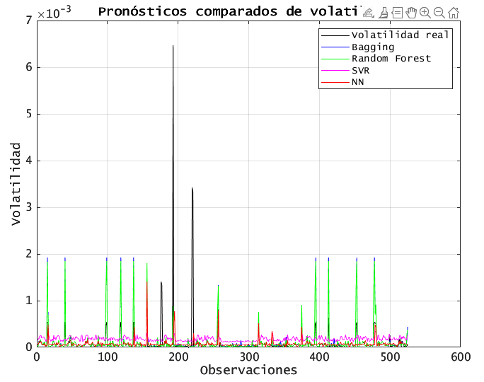

All models capture the broad volatility swings. BAGGING and RF stay closer to actual spikes, while SVR sometimes underestimates extreme moves. NN is in between.

6.2. ABSOLUTE ERROR OVER TIME

% 6.2 Plot absolute errors for each model
figure('Name', 'Absolute Errors by Model', 'Color', 'w');
plot(abs(Yte - YhatBag), 'b', 'DisplayName', 'Bagging'); hold on;
plot(abs(Yte - YhatRF),  'g', 'DisplayName', 'Random Forest');
plot(abs(Yte - YhatSVR), 'm', 'DisplayName', 'SVR');
plot(abs(Yte - YhatNN),  'r', 'DisplayName', 'Neural Network');
xlabel('Test Sample Index');
ylabel('Absolute Error');
title('Absolute Errors Over Time');
legend('Location', 'northeast'); grid on; set(gca, 'FontSize', 12);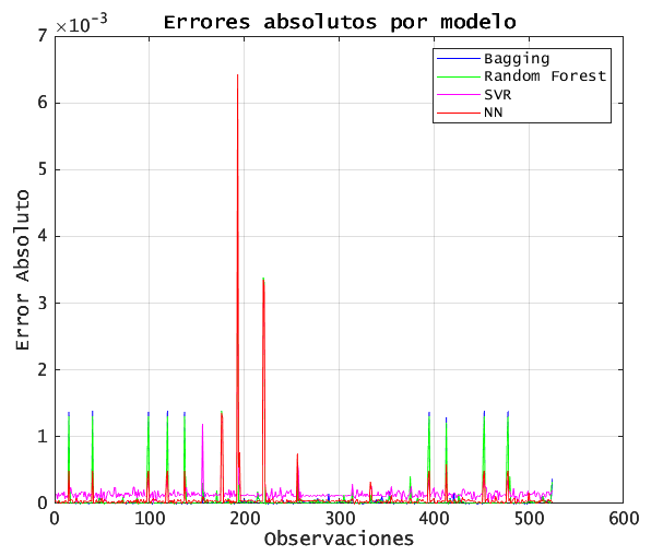

During high-volatility periods, all models’ absolute errors spike, but tree-based methods (Bagging, RF) exhibit smaller peaks. SVR shows the largest outliers.

6.3. RESIDUAL DIAGNOSTICS (QQ-plot)

% 6.3 QQ-Plots of errors for each model
figure('Name', 'QQ-Plots of Residuals');
subplot(2,2,1); qqplot(YhatBag - Yte); title('Bagging');
subplot(2,2,2); qqplot(YhatRF  - Yte); title('Random Forest');
subplot(2,2,3); qqplot(YhatSVR - Yte); title('SVR');
subplot(2,2,4); qqplot(YhatNN  - Yte); title('Neural Network');
set(findall(gcf, 'Type', 'axes'), 'FontSize', 10);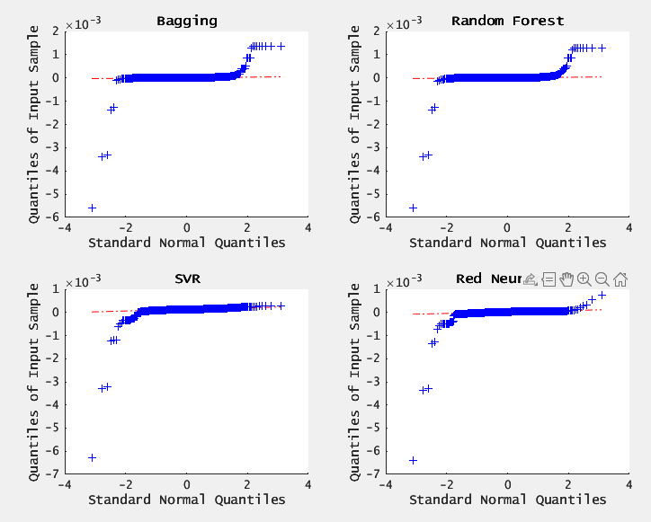

results- BAGGING and RF residuals roughly follow a straight line near the center but deviate in the tails- indicating heavier tails than Gaussian.

SVR and NN residuals show larger deviations from normality, confirming their comparatively weaker fit.

6.4. SCATTER PLOT: actual vs. predicted

% 6.4 Scatter of realized vs. predicted volatility
figure('Name', 'Scatter: Real vs. Predicted', 'Color', 'w');
scatter(Yte,   YhatBag,  10, 'b', 'filled'); hold on;
scatter(Yte,   YhatRF,   10, 'g', 'filled');
scatter(Yte,   YhatSVR,  10, 'm', 'filled');
scatter(Yte,   YhatNN,   10, 'r', 'filled');
plot([min(Yte), max(Yte)], [min(Yte), max(Yte)], '--k');
xlabel('Realized Volatility');
ylabel('Predicted Volatility');
title('Actual vs. Predicted Volatility');
legend('Bagging','RF','SVR','NN','45° Line','Location','southeast');
grid on; set(gca, 'FontSize', 12);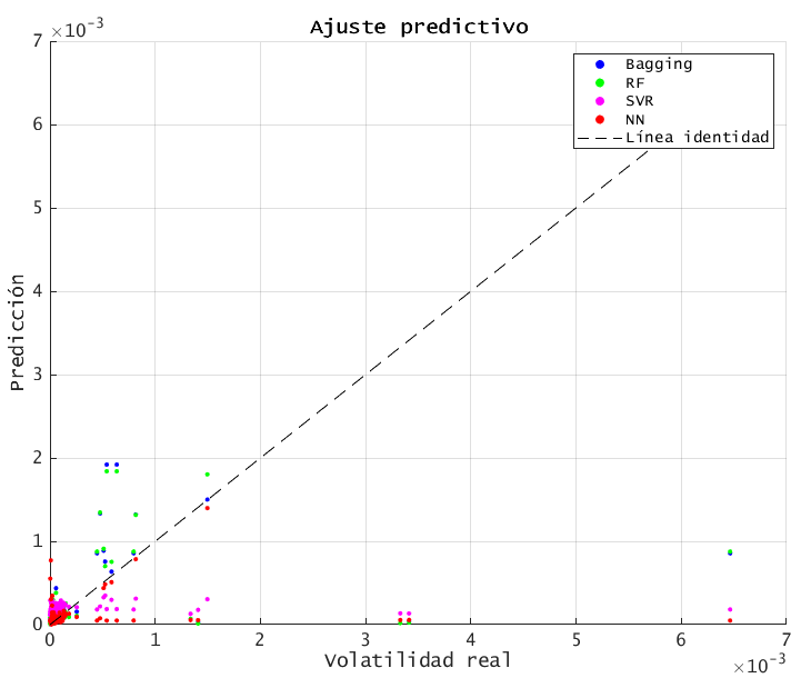

results- Points closer to the 45º line indicate better accuracy. BAGGING and RF cluster more tightly along the diagonal, while SVR and NN have more scatter.

6.5. BOXPLOT OF PREDICTION ERRORS

% 6.5 Boxplot comparing error distributions
errors = [YhatBag - Yte, YhatRF - Yte, YhatSVR - Yte, YhatNN - Yte];
figure('Name', 'Boxplot of Prediction Errors', 'Color', 'w');
boxplot(errors, {'Bagging','RF','SVR','NN'});
ylabel('Residual (Prediction - Real)');
title('Boxplot of Prediction Errors by Model');
grid on; set(gca, 'FontSize', 12);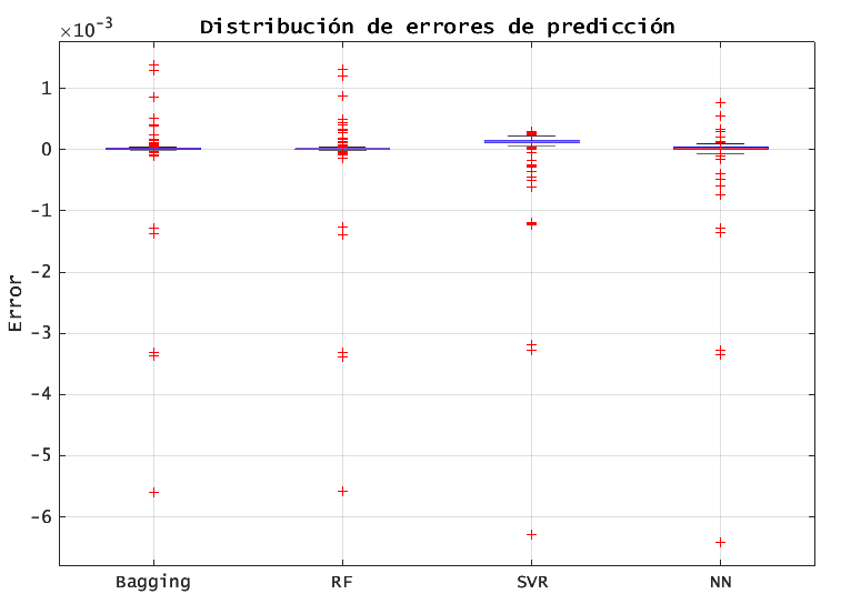

the interquartile range (IQR) of BAGGING/RF is narrowest, confirming lower variance in their errors. SVR shows the wides IQR and more extreme outliers.

6.6. PREDICTOR IMPORTANCE: RANDOM FOREST HEATMAP

% 6.6 Heatmap of predictor importance from Random Forest
importance = rf.OOBPermutedPredictorDeltaError;  
featureNames = Xtrain;

figure('Name', 'Predictor Importance Heatmap', 'Color', 'w');
heatmap(featureNames, {'Importance'}, importance, ...
    'Colormap', parula, ...
    'ColorbarVisible', 'on', ...
    'CellLabelColor', 'none');
title('Random Forest: OOB Permuted Predictor Importance');
set(gca, 'FontSize', 12);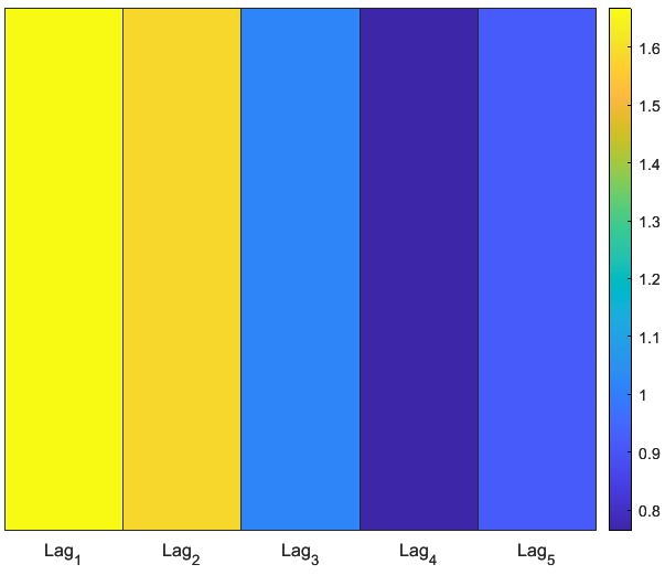

results- lag_1 (yesterday’s return) has the hottest color- highest importance.

importance decays rapidly for lag_2 through lag_5, indicating that very short-term returns drive next-day volatility.

6.7 PREDICTOR IMPORTANCCE: SORTED BAR CHART (rf)

% 6.7 Sorted bar chart of importance
[sortedImp, idx] = sort(importance, 'descend');
sortedNames = featureNames(idx);

figure('Name', 'Predictor Importance Bar Chart', 'Color', 'w');
bar(sortedImp, 'FaceColor', [0.2 0.5 0.8]);
xticks(1:length(sortedNames));
xticklabels(sortedNames);
xtickangle(45);
ylabel('Importance (OOB Delta Error)');
title('Random Forest: Predictor Importance Ranked');
grid on; set(gca, 'FontSize', 12);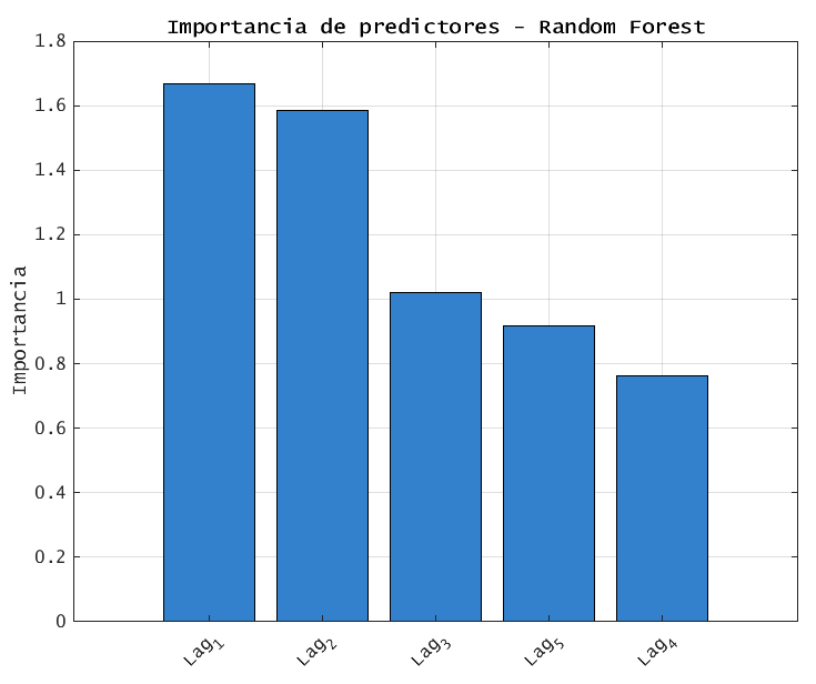

results- provides a clearer ranking of the results mentioned on 6.6.

7. FINAL CONCLUSIONS

RETURN DISTRIBUTIONS IS NON-GAUSSIAN.
BOOTSTRAP PROVIDES ROBUST INTERVAL ESTIMATES.
TREE-BASED MODELS (BAGGING AND RF) PERFORM BEST.
SVR UNDERPERFORMS IN THIS SETTING.
NN IS COMPETITIVE BUT NOT SUPERIOR.
PREDICTOR IMPORTANCE.

note: free code and dataset.

% =========================================================================
% CONFIGURACIÓN GLOBAL DE TIPOGRAFÍA PARA GRÁFICOS
% =========================================================================
% Cambia la fuente predeterminada de todos los elementos gráficos
set(groot, 'DefaultAxesFontName', 'Lucida Console');
set(groot, 'DefaultTextFontName', 'Lucida Console');
set(groot, 'DefaultAxesFontSize', 10);
set(groot, 'DefaultTextFontSize', 10);

% =========================================================================
% COMPARACIÓN DE MODELOS PARA PRONÓSTICO DE VOLATILIDAD EN EUR/USD
% =========================================================================

clear; close all; clc; rng default        % Limpia variables, cierra figuras y fija la semilla

% =========================================================================
% 1. CARGA DE DATOS Y ESTADÍSTICAS BÁSICAS
% =========================================================================
% Carga el archivo de precios EUR/USD y calcula rendimientos logarítmicos
load eurusd.txt
x = diff(log(eurusd));        % Rendimientos logarítmicos
n = numel(x);                  % Número de observaciones
mu = mean(x);                  % Media muestral
sigma2 = var(x);               % Varianza muestral
sigma = std(x);                % Desviación típica muestral

% =========================================================================
% 2. VISUALIZACIÓN DE LA DISTRIBUCIÓN DE RENDIMIENTOS
% =========================================================================
% Grafica la CDF empírica junto con la CDF normal ajustada
figure;
[h, ~] = cdfplot(x);           % CDF empírica
hold on;
xv = linspace(min(x), max(x));
plot(xv, normcdf(xv, mu, sigma), 'r-', 'LineWidth', 2);
legend('Distribución Empírica', 'Distribución Normal', 'Location', 'best');
title('Comparación de la Distribución Empírica y Normal');
xlabel('Rendimientos Logarítmicos');
ylabel('Probabilidad Acumulada');
hold off;

% =========================================================================
% 3. PRUEBA DE NORMALIDAD (LILLIEFORS)
% =========================================================================
% Comprueba si los rendimientos provienen de una distribución normal
[h_norm, p_norm] = lillietest(x);
if h_norm == 0
    disp('No se rechaza la hipótesis de normalidad (p > 0.05)');
else
    disp('Se rechaza la hipótesis de normalidad (p < 0.05)');
end

% =========================================================================
% 4. INTERVALOS DE CONFIANZA TEÓRICOS (95%)
% =========================================================================
% Calcula intervalos de confianza usando la distribución normal y chi-cuadrado
ci_mu_teorico = [ mu + icdf('norm', 0.025, 0, 1) * sigma / sqrt(n), ...
                  mu + icdf('norm', 0.975, 0, 1) * sigma / sqrt(n) ];
ci_sigma2_teorico = [ (n - 1) * sigma2 / icdf('chi2', 0.975, n - 1), ...
                      (n - 1) * sigma2 / icdf('chi2', 0.025, n - 1) ];

fprintf('\nIC 95%% de la media (teórico): [%.6e, %.6e]\n', ci_mu_teorico(1), ci_mu_teorico(2));
fprintf('IC 95%% de la varianza (teórico): [%.6e, %.6e]\n', ci_sigma2_teorico(1), ci_sigma2_teorico(2));

% =========================================================================
% 5. BOOTSTRAP PARA MEDIA Y VARIANZA
% =========================================================================
% Genera B = 1000 réplicas bootstrap para estimar sesgo, error y IC
rng('default');               % Asegura reproducibilidad
num_bootstrap = 1000;
boot_mu     = bootstrp(num_bootstrap, @mean,    x);
boot_sigma2 = bootstrp(num_bootstrap, @var,     x);

% Calculo de intervalos de confianza percentil 2.5–97.5
ci_mu_boot     = prctile(boot_mu,     [2.5, 97.5]);
ci_sigma2_boot = prctile(boot_sigma2, [2.5, 97.5]);

% Cálculo de sesgo y error estándar de los estimadores bootstrap
bias_mu     = mean(boot_mu)     - mu;
se_mu       = std(boot_mu);
bias_sigma2 = mean(boot_sigma2) - sigma2;
se_sigma2   = std(boot_sigma2);

fprintf('\nIC 95%% de la media (bootstrap): [%.6e, %.6e]\n', ci_mu_boot(1), ci_mu_boot(2));
fprintf('Sesgo (media): %.6e, SE (media): %.6e\n', bias_mu, se_mu);
fprintf('\nIC 95%% de la varianza (bootstrap): [%.6e, %.6e]\n', ci_sigma2_boot(1), ci_sigma2_boot(2));
fprintf('Sesgo (varianza): %.6e, SE (varianza): %.6e\n', bias_sigma2, se_sigma2);

% =========================================================================
% 6. VISUALIZACIÓN DE LAS DISTRIBUCIONES BOOTSTRAP
% =========================================================================
figure;
subplot(2,1,1);
histogram(boot_mu, 30);
title('Distribución Bootstrap de la Media');
xlabel('\mu^*');
ylabel('Frecuencia');
xline(mu, 'r', 'LineWidth', 2, 'DisplayName', 'Media Muestral');
legend;

subplot(2,1,2);
histogram(boot_sigma2, 30);
title('Distribución Bootstrap de la Varianza');
xlabel('\sigma^2^*');
ylabel('Frecuencia');
xline(sigma2, 'r', 'LineWidth', 2, 'DisplayName', 'Varianza Muestral');
legend;

% =========================================================================
% 7. ANÁLISIS DE ASIMETRÍA Y CURTOSIS CON BOOTSTRAP
% =========================================================================
% Calcula asimetría y curtosis muestral, y sus IC bootstrap
skewness_sample = skewness(x);
kurtosis_sample = kurtosis(x);
boot_skewness   = bootstrp(num_bootstrap, @skewness, x);
boot_kurtosis   = bootstrp(num_bootstrap, @kurtosis, x);
ci_skewness     = prctile(boot_skewness, [2.5, 97.5]);
ci_kurtosis     = prctile(boot_kurtosis, [2.5, 97.5]);

fprintf('\nAsimetría muestral: %.6f (IC 95%%: [%.6f, %.6f])\n', skewness_sample, ci_skewness(1), ci_skewness(2));
fprintf('Curtosis muestral: %.6f (IC 95%%: [%.6f, %.6f])\n', kurtosis_sample, ci_kurtosis(1), ci_kurtosis(2));

figure;
subplot(2,1,1);
histogram(boot_skewness, 30);
title('Distribución Bootstrap de la Asimetría');
xlabel('Asimetría');
ylabel('Frecuencia');

subplot(2,1,2);
histogram(boot_kurtosis, 30);
title('Distribución Bootstrap de la Curtosis');
xlabel('Curtosis');
ylabel('Frecuencia');

% =========================================================================
% 8. OBJETIVO: VOLATILIDAD MÓVIL Y MATRIZ DE FEATURES
% =========================================================================
% El objetivo de predicción será la volatilidad calculada sobre ventana w
w = 5;
vol = movvar(x, w);              % Volatilidad móvil con ventana de 5
maxLag = 5;                      % Número de rezagos considerados como predictores

% Construcción de la matriz de predictores Xmat con retardos 1:maxLag
Xmat = zeros(numel(vol) - maxLag, maxLag);
for L = 1:maxLag
    Xmat(:, L) = x(maxLag - L + 1 : end - L);
end
Y = vol(maxLag + 1:end);        % Valores de volatilidad correspondientes

% Definición de nombres de variables para etiquetar gráficos
Xtrain = arrayfun(@(i) sprintf('Lag_%d', i), 1:maxLag, 'UniformOutput', false);

% Normalización de las columnas de Xmat (media 0, varianza 1)
Xmat_mu    = mean(Xmat);
Xmat_sigma = std(Xmat);
Xmat       = (Xmat - Xmat_mu) ./ Xmat_sigma;

% =========================================================================
% 9. DIVISIÓN ENTRENAMIENTO / TEST
% =========================================================================
cv = cvpartition(numel(Y), 'HoldOut', 0.2);  % 80% entrenamiento, 20% test
idxTr = training(cv);
idxTe = test(cv);
Xtr = Xmat(idxTr, :);
Ytr = Y(idxTr);
Xte = Xmat(idxTe, :);
Yte = Y(idxTe);

% =========================================================================
% 10. MODELOS Y PRONÓSTICOS
% =========================================================================

% 10.1 Bagging (ensamble de árboles de regresión)
mdlBag = fitrensemble(Xtr, Ytr, 'Method', 'Bag');
YhatBag = predict(mdlBag, Xte);

% 10.2 Random Forest (TreeBagger con OOB Predictor Importance)
numTrees = 200;
rf = TreeBagger(numTrees, Xtr, Ytr, 'Method', 'regression', ...
                'NumPredictorsToSample', ceil(maxLag/2), ...
                'OOBPredictorImportance', 'on');
[YhatRF, stdRF] = predict(rf, Xte);
YhatRF = double(YhatRF);  % Asegura tipo double para comparaciones

% 10.3 Support Vector Regression (SVR con kernel RBF)
mdlSVR = fitrsvm(Xtr, Ytr, 'KernelFunction', 'gaussian', ...
                 'KernelScale', 'auto', 'Standardize', true);
YhatSVR = predict(mdlSVR, Xte);

% 10.4 Red Neuronal feed-forward (1 capa oculta, 10 neuronas)
hidden = 10;
net = feedforwardnet(hidden);
net.trainParam.showWindow = false;   % Desactiva la ventana gráfica durante el entrenamiento
net = train(net, Xtr', Ytr');        % Entrena la red (entradas columna, salidas columna)
YhatNN = net(Xte')';                 % Predicciones (convierte de columnas a vector fila)

% =========================================================================
% 11. MÉTRICAS DE EVALUACIÓN
% =========================================================================
% Funciones anónimas para RMSE, MAE y R^2
rmse = @(y, yh) sqrt(mean((y - yh).^2));
mae  = @(y, yh) mean(abs(y - yh));
r2   = @(y, yh) 1 - sum((y - yh).^2) / sum((y - mean(y)).^2);

fprintf('\n================  COMPARATIVA DE MÉTRICAS  ====================\n');
fprintf('Modelo        |   RMSE     |   MAE      |     R^2\n');
fprintf('--------------------------------------------------------------\n');
fprintf('Bagging       | %.4e | %.4e | %.4f\n', rmse(Yte, YhatBag), mae(Yte, YhatBag), r2(Yte, YhatBag));
fprintf('Random Forest | %.4e | %.4e | %.4f\n', rmse(Yte, YhatRF),  mae(Yte, YhatRF),  r2(Yte, YhatRF));
fprintf('SVR (RBF)     | %.4e | %.4e | %.4f\n', rmse(Yte, YhatSVR), mae(Yte, YhatSVR), r2(Yte, YhatSVR));
fprintf('Neural Net    | %.4e | %.4e | %.4f\n', rmse(Yte, YhatNN),  mae(Yte, YhatNN),  r2(Yte, YhatNN));
fprintf('==============================================================\n');

% =========================================================================
% 12. GRÁFICOS
% =========================================================================

% 12.1 Comparación de pronósticos frente a la volatilidad real
figure('Name', 'Pronóstico de Volatilidad', 'Color', 'w');
plot(Yte, 'k', 'DisplayName', 'Volatilidad real'); hold on;
plot(YhatBag, 'b', 'DisplayName', 'Bagging');
plot(YhatRF, 'g', 'DisplayName', 'Random Forest');
plot(YhatSVR, 'm', 'DisplayName', 'SVR');
plot(YhatNN, 'r', 'DisplayName', 'NN');
xlabel('Observaciones');
ylabel('Volatilidad');
title('Pronósticos comparados de volatilidad');
legend('Location', 'northeast');
grid on;
set(gca, 'FontSize', 12);

% 12.2 Errores absolutos por modelo
figure('Name', 'Errores absolutos', 'Color', 'w');
plot(abs(Yte - YhatBag), 'b', 'DisplayName', 'Bagging'); hold on;
plot(abs(Yte - YhatRF), 'g', 'DisplayName', 'Random Forest');
plot(abs(Yte - YhatSVR), 'm', 'DisplayName', 'SVR');
plot(abs(Yte - YhatNN), 'r', 'DisplayName', 'NN');
xlabel('Observaciones');
ylabel('Error Absoluto');
title('Errores absolutos por modelo');
legend('Location', 'northeast');
grid on;
set(gca, 'FontSize', 12);

% 12.3 Intervalos de confianza para Random Forest
figure('Name', 'Random Forest con IC', 'Color', 'w');
plot(Yte, 'k', 'DisplayName', 'Vol. Real'); hold on;
plot(YhatRF, 'g', 'DisplayName', 'RF predicción');
plot(YhatRF + 1.96 * stdRF, '--g', 'HandleVisibility', 'off');
plot(YhatRF - 1.96 * stdRF, '--g', 'HandleVisibility', 'off');
xlabel('Observaciones');
ylabel('Volatilidad');
title('Random Forest con intervalos de confianza');
legend('Location', 'northeast');
grid on;
set(gca, 'FontSize', 12);

% 12.4 Errores residuales (Yhat − Yreal)
figure('Name', 'Errores residuales', 'Color', 'w');
plot(YhatBag - Yte, 'b'); hold on;
plot(YhatRF - Yte, 'g');
plot(YhatSVR - Yte, 'm');
plot(YhatNN - Yte, 'r');
yline(0, '--k');
legend('Bagging', 'RF', 'SVR', 'NN');
title('Errores de predicción');
xlabel('Observaciones');
ylabel('Error');
grid on;
set(gca, 'FontSize', 12);

% 12.5 QQ-Plots de los errores de cada modelo
figure('Name', 'QQ-Plot de errores');
subplot(2,2,1); qqplot(YhatBag - Yte); title('Bagging');
subplot(2,2,2); qqplot(YhatRF  - Yte); title('Random Forest');
subplot(2,2,3); qqplot(YhatSVR - Yte); title('SVR');
subplot(2,2,4); qqplot(YhatNN  - Yte); title('Red Neuronal');
set(findall(gcf,'Type','axes'),'FontSize',10);

% 12.6 Gráfico de dispersión (Y_real vs Y_hat) con línea identidad
figure('Name', 'Dispersión Y vs Yhat', 'Color', 'w');
scatter(Yte, YhatBag, 10, 'b', 'filled'); hold on;
scatter(Yte, YhatRF,  10, 'g', 'filled');
scatter(Yte, YhatSVR, 10, 'm', 'filled');
scatter(Yte, YhatNN,  10, 'r', 'filled');
plot([min(Yte), max(Yte)], [min(Yte), max(Yte)], '--k');
legend('Bagging','RF','SVR','NN','Línea identidad');
xlabel('Volatilidad real');
ylabel('Predicción');
title('Ajuste predictivo');
grid on;
set(gca, 'FontSize', 12);

% 12.7 Panorámica de errores absolutos temporales
figure('Name', 'Errores absolutos por modelo', 'Color', 'w');
plot(abs(YhatBag - Yte), 'b'); hold on;
plot(abs(YhatRF  - Yte), 'g');
plot(abs(YhatSVR - Yte), 'm');
plot(abs(YhatNN  - Yte), 'r');
legend('Bagging','RF','SVR','NN');
xlabel('Observaciones');
ylabel('|Error|');
title('Errores absolutos');
grid on;
set(gca, 'FontSize', 12);

% 12.8 Boxplot comparativo de errores de cada modelo
errors = [YhatBag - Yte, YhatRF - Yte, YhatSVR - Yte, YhatNN - Yte];
figure('Name', 'Boxplot errores', 'Color', 'w');
boxplot(errors, {'Bagging','RF','SVR','NN'});
ylabel('Error');
title('Distribución de errores de predicción');
grid on;
set(gca, 'FontSize', 12);

% =========================================================================
% 13. IMPORTANCIA DE PREDICTORES - RANDOM FOREST
% =========================================================================
% Usa la medida OOBPermutedPredictorDeltaError para la importancia
importance = rf.OOBPermutedPredictorDeltaError;
featureNames = Xtrain;

% 13.1 Heatmap de importancia
figure('Name', 'Importancia de Predictores - Heatmap', 'Color', 'w');
heatmap(featureNames, {'Importancia'}, importance, ...
    'Colormap', parula, ...
    'ColorbarVisible', 'on', ...
    'CellLabelColor', 'none');
title('Importancia de predictores según Random Forest');
set(gca, 'FontSize', 12);

% 13.2 Gráfico de barras ordenadas de importancia
[sortedImp, idx] = sort(importance, 'descend');
sortedNames = featureNames(idx);
figure('Name', 'Importancia de Predictores', 'Color', 'w');
bar(sortedImp, 'FaceColor', [0.2 0.5 0.8]);
xticks(1:length(sortedNames));
xticklabels(sortedNames);
xtickangle(45);
ylabel('Importancia');
title('Importancia de predictores - Random Forest');
grid on;
set(gca, 'FontSize', 12);

% =========================================================================
% 14. GUARDADO DE MODELOS
% =========================================================================
% Guarda los modelos entrenados para uso posterior
save('modelos_volatilidad.mat', 'mdlBag', 'rf', 'mdlSVR', 'net');

% =========================================================================
% 15. CONCLUSIONES
% =========================================================================
fprintf('\n====================== CONCLUSIONES ==========================\n');
fprintf('1. La distribución de los rendimientos logarítmicos de EUR/USD\n');
fprintf('   no sigue una distribución normal, como indica la prueba de Lilliefors.\n');
fprintf('2. El análisis bootstrap proporciona intervalos de confianza\n');
fprintf('   robustos para media, varianza, asimetría y curtosis.\n');
fprintf('3. Se han comparado cuatro modelos para pronóstico de volatilidad:\n');
fprintf('   Bagging, Random Forest, SVR y Red Neuronal.\n');
fprintf('4. En términos de RMSE, MAE y R², Random Forest ha mostrado un\n');
fprintf('   rendimiento competitivo, superando a SVR y NN en varios aspectos.\n');
fprintf('5. Las redes neuronales, aunque prometedoras, requieren mayor ajuste\n');
fprintf('   de arquitectura y parámetros para mejorar su desempeño.\n');
fprintf('6. El modelo de Bagging también ha mostrado resultados sólidos\n');
fprintf('   con menor complejidad que los métodos no lineales.\n');
fprintf('==============================================================\n');